Quench dynamics in integrable models
from the Quench Action
to renormalization from integrability
Great Lessons from Exact Techniques and Beyond
Tropea, 29 August 2023Jean-Sébastien Caux


Plan of the talk
The Lieb-Liniger Model
$ H = \int_0^L dx \left[ \partial_x \Psi^{\dagger}(x) \partial_x \Psi(x) + c \Psi^{\dagger} (x) \Psi^{\dagger}(x) \Psi(x) \Psi(x) \right] $
Eigenstates: Bethe Ansatz
\[ \begin{align} \Psi_N(\{ x \} | \{ \lambda \}) &= \prod_{N \geq j_1 > j_2 \geq 1} sgn(x_{j_1} - x_{j_2}) sgn (\lambda_{j_1} - \lambda_{j_2}) \times \\ &\times \sum_{P \in \pi_N} (-1)^{[P]} e^{i \sum_{j=1}^N \lambda_{P_j} x_j + \frac{i}{2} \sum_{N \geq j_1 > j_2 \geq 1} sgn(x_{j_1} - x_{j_2}) \phi (\lambda_{P_{j_1}} - \lambda_{P_{j_2}})} \end{align} \]
in which $\phi(\lambda) \equiv 2\mbox{atan}(\lambda/c)$
The Lieb-Liniger Model
Rapidities must obey the Bethe equations:
$ e^{\mathrm{i}\lambda_j L} = \prod_{\substack{{\tiny l=1} \\ {\tiny (l\neq j)}}}^{\tiny N} \frac{ \lambda_j - \lambda_l + \mathrm{i}c}{\lambda_j - \lambda_l - \mathrm{i}c} $
Eigenvalues of conserved charges:
$ Q_n\left(\{\lambda\}_N\right) = \sum_{j=1}^N \lambda_j^n, \quad n = 1,2,\ldots $
with in particular $P = Q_1, E = Q_2$.
The Lieb-Liniger Model
Description using the Algebraic Bethe Ansatz
\[ \tau(\lambda) = tr T(\lambda), \hspace{5mm} T(\lambda) = \left( \begin{array}{cc} A(\lambda) & B(\lambda) \\ C(\lambda) & D(\lambda) \end{array} \right), \hspace{5mm} | \Psi_N \left( \left\{ \lambda \right\}_N \right \rangle = \prod_j B(\lambda_j) | 0 \rangle \]
Matrix elements of physical operators known from:
- Gaudin formula for state norm
\[ \langle \{ \lambda \} | \{ \lambda \} \rangle = c^N \prod_{j > k} \frac{\lambda_{jk}^2 + c^2}{\lambda_{jk}^2} \mbox{det} \left[ \delta_{jk} \left(L + \sum_l K_{jl} \right) - K_{jk} \right], \hspace{10mm} K_{jk} = \frac{2c}{\lambda_{jk}^2 + c^2} \]
- solution of inverse problem $A, B, C, D \leftrightarrow \psi(x), \psi^\dagger(x)$
- Slavnov formula for $\langle 0 | \prod_j C(\lambda_j) \prod_k B(\mu_k) | 0 \rangle$
The Lieb-Liniger Model
(Dynamical) Correlation functions
\[ {\cal S}^{a \bar{a}} (k, \omega) \equiv \frac{1}{N} \sum_{j, j'} e^{-i k(j-j')} \int_{-\infty}^\infty dt e^{i\omega t} \langle \frac{1}{2} \left[ {\cal O}^a_j (t), ({\cal O}^a_{j'} (0))^\dagger \right] \rangle \]
Simplest examples:
- Dynamical structure factor: ${\cal O}_j = \rho_j \equiv \Psi^\dagger(x_j) \Psi(x_j)$
- One-body function (Green's): ${\cal O}_j = \Psi(x_j)$ or $\Psi^\dagger(x_j)$
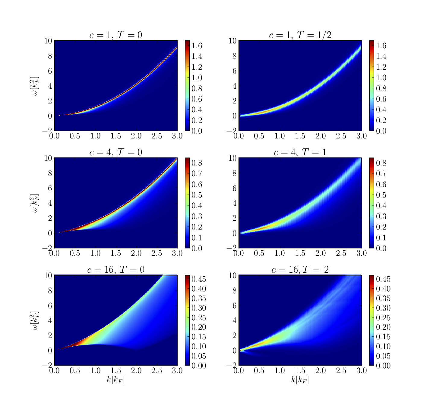
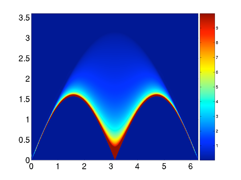
Dynamical structure factor
from (algebraic) Bethe Ansatz
The ABACUS algorithm
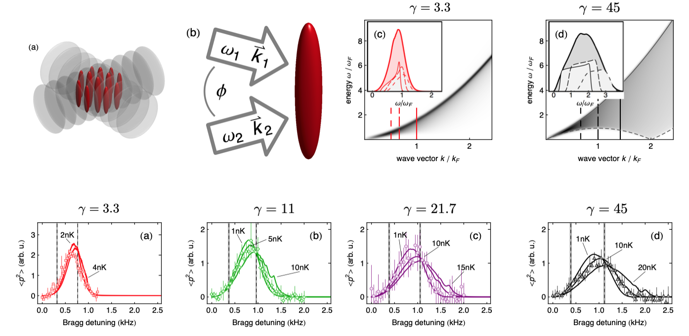
Dynamical structure factor from Bethe Ansatz
extension to finite TM. Panfil and J-SC, PRA 89 (2014)
Lieb-Liniger using cold atoms (I)
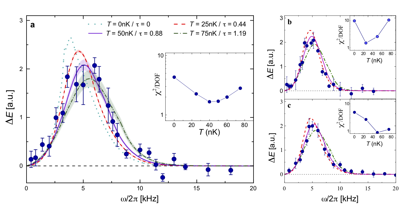
Lieb-Liniger using cold atoms (II)
What we really would like to do with exact methods
- Beyond linear response
- Quenches
- Driving
Out-of-equilibrium using Integrability
- The super Tonks-Girardeau gas
- Split Fermi seas (Moses states)
- Spin echo in quantum dots
- Quasisolitons
- Interaction quench in Richardson
- Domain wall release in Heisenberg
- Geometric quench
- Interaction cutoff in Lieb-Liniger
- Release of trapped Lieb-Liniger
- BEC to Lieb-Liniger quench
- Quantum Newton’s Cradle in TG
- Néel to XXZ quench
- Generalized hydrodynamics
- Floquet driven spin chains
Quenches
Interaction quench in Lieb-Liniger
We will consider a sudden switch of the interaction:
$ c (t) = \left\{ \begin{array}{ll} c_i & t < 0, \\ c_f & t > 0 \end{array} \right. $
starting in ground/(any eigen)state of $H(c_i)$ at $t < 0$
For many reasons, this is a complicated problem...
- GGE logic fails, charges have $\infty$ exp. values
- approaches using regularizations (q-bosons, extended charges, ...): no complete solution
The strategy
We write the initial state in the basis of the eigenstates of $H(c_f)$, denoted as $\left\{ |\{\lambda\}^{(n)}_N\rangle \right\}, n = 0, 1, ...$
The initial state is obtained as a linear decomposition weighed by exact overlaps:
$ |\Psi_i\rangle = \sum_{n=0}^\infty |\{\lambda\}^{(n)}_N\rangle \underbrace{\langle \{\lambda\}^{(n)}_N | \Psi_i\rangle}_{\text{the overlaps}} $
Exact time-evolved state:
$ |\Psi_i(t)\rangle \equiv e^{-iH(c_f)t} |\Psi_i\rangle = \sum_{n=0}^\infty e^{-\mathrm{i}E(\{\lambda\}^{(n)}_N)t} |\{\lambda\}^{(n)}_N\rangle \langle \{\lambda\}^{(n)}_N | \Psi_i\rangle $
The Quench Action
Setup
The initial state is decomposed in the basis of post-quench Hamiltonian eigenstates:
$ |\Psi (t=0) \rangle = \sum_{\{ I \}} e^{-S^\Psi_{\{ I \}}} | \{ I \} \rangle, $
with overlaps encoded in the coefficients$ S^\Psi_{\{ I \}} = -\ln \langle \{ I \} | \Psi (t=0) \rangle ~\in ~\mathbb{C} $
Exact time-dependend expectation values:
$ \bar{\cal O} (t) = \frac{ \sum_{\{ I^l \} } \sum_{\{ I^r\}} e^{-(S^\Psi_{\{ I^l\}})^* - S^\Psi_{\{ I^r\}} + i (\omega_{\{ I^l\}} - \omega_{\{ I^r\}})t} \langle \{ I^l \}| {\cal O} | \{ I^r \} \rangle}{\sum_{\{ I \}} e^{-2\Re S^\Psi_{\{ I \}}}} $
Going to the thermodynamic limit
Summations over eigenstates are replaced by functional integrals
$ \lim_{Th,reg} \sum_{\{ \rho_i \}} (...) = \int_{\rho_{sm} \in C^\infty} D\rho_{sm} (...) $
Normalization sum (trivially 1) represented as
$ \lim_{Th,reg} \langle \Psi (t) | \Psi (t) \rangle = \int D\rho_{sm} ~ e^{-S^Q[\rho_{sm}]} $
where the Quench Action is defined as
$ S^{Q}[\rho] = S^o[\rho] - S^{YY}[\rho] $
Time-dependent expectation values
In ThLim, saddle-point evaluation $\left. \frac{\delta S^Q[\rho]}{\delta \rho} \right|_{\rho_{sp}} = 0$ exactly gives the full time evolution of observables as
$ \begin{align} \lim_{Th,reg} \bar{\cal O} (t) = \lim_{Th,reg} \frac{1}{2} \sum_{\bf e} \left[ e^{-\delta S_{\bf e}[\rho_{sp}] - i \omega_{\bf e}[\rho_{sp}] t} \langle \rho_{sp} | {\cal O} | \rho_{sp}; {\bf e} \rangle \right. \nonumber \\ \left. + e^{-\delta S^*_{\bf e}[\rho_{sp}] + i \omega_{\bf e}[\rho_{sp}] t} \langle \rho_{sp}; {\bf e} | {\cal O} | \rho_{sp} \rangle \right] \end{align} $
provided the
operator ${\cal O}$ is
- weak
- smooth
- thermodynamically finite
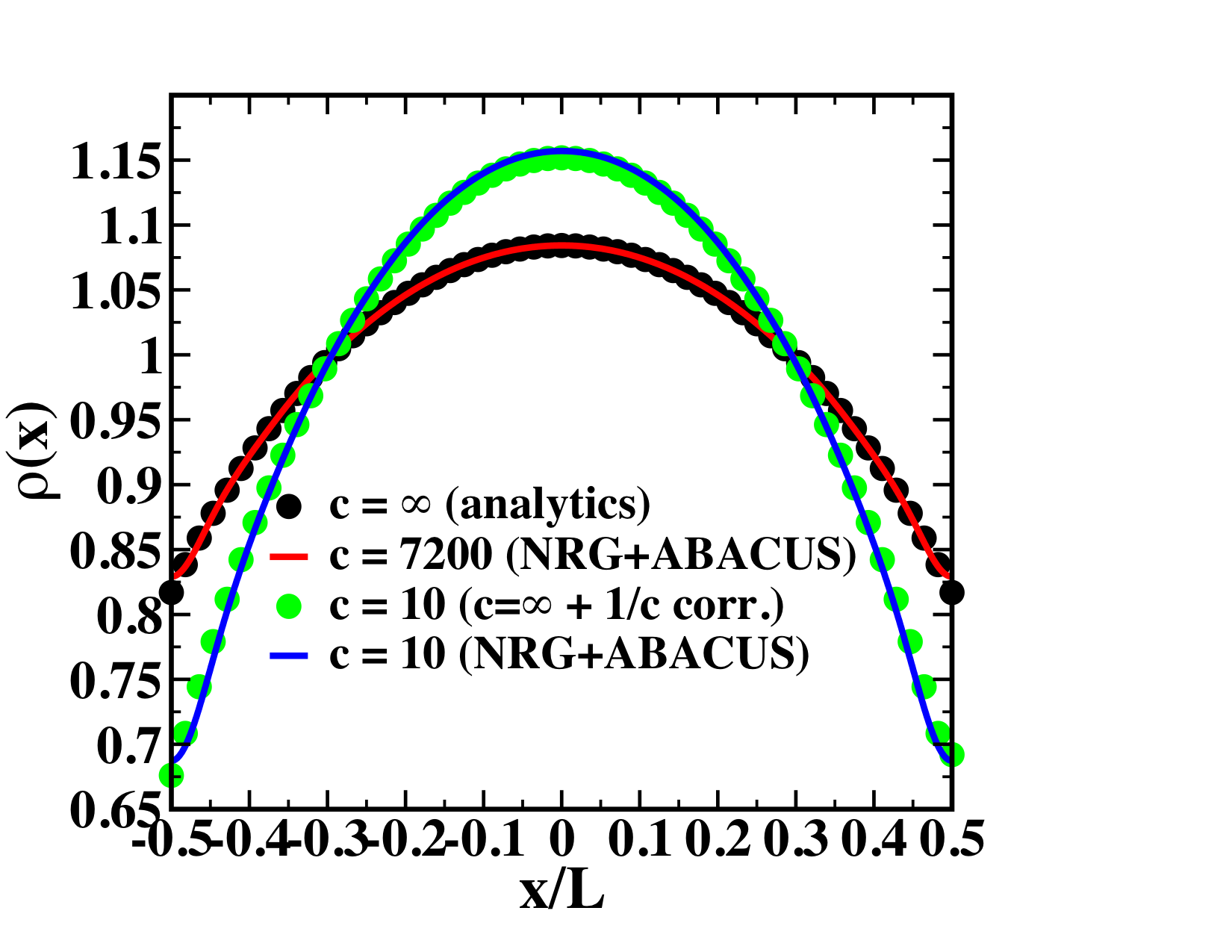
The BEC to Lieb-Liniger quench
Initial state: ground state of free bosons
$ | \Psi_0 \rangle = \frac{1}{\sqrt{L^N N!}} \left(\psi_{k=0}^\dagger\right)^N | 0 \rangle $
Exact overlaps with finite $c$ Lieb-Liniger states:
$ \langle \Psi_0 | \{ \lambda \}_{N/2} \cup \{ -\lambda \}_{N/2} \rangle = \left[ \frac{(cL)^{-N} N!}{\mbox{det}_N G_{jk} }\right]^{1/2} \frac{\mbox{det}_{N/2} G^Q_{jk}}{\prod_{j=1}^{N/2} \frac{\lambda_j}{c} \left[ \frac{\lambda_j^2}{c^2} + \frac{1}{4} \right]^{1/2}} $
in which $G_{jk}$ is the Gaudin matrix
$ G_{jk} = \delta_{jk} \left[ L + \sum_{l=1}^N K (\lambda_j, \lambda_l) \right] - K(\lambda_j, \lambda_k) $
Exact solution using Quench Action
$ S^Q = L\int_0^\infty d\lambda \rho(\lambda) \log\left(\frac{\lambda^2}{c^2} \left( \frac{1}{4} + \frac{ \lambda^2}{c^2} \right) \right) + S^{YY} $
Saddle-point equation:
$ \ln \eta(\lambda) = g(\lambda) - h - \int_{-\infty}^\infty \frac{d\lambda'}{2\pi} K (\lambda - \lambda') \ln \left[ 1 + \eta^{-1}(\lambda') \right], $
with driving term $ g(\lambda) = \ln \left[ \frac{\lambda^2}{c^2} \left( \frac{\lambda^2}{c^2} + \frac{1}{4} \right) \right] $
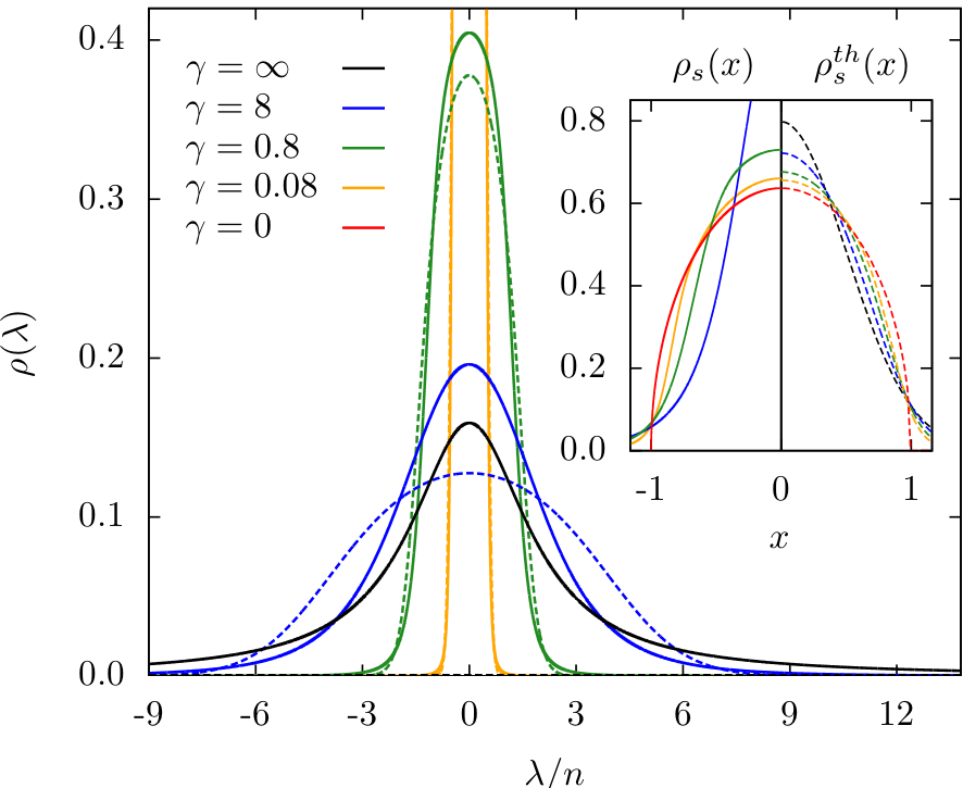
Analytic solution for steady state:
$ \begin{align} \rho_{sp} (\lambda) &= -\frac{\gamma}{4\pi} \frac{1}{1 + a(\lambda)} \frac{\partial a(\lambda)}{\partial \gamma},\\ a(\lambda) &\equiv \frac{2\pi}{\frac{\lambda}{n} \sinh \frac{2\pi \lambda}{c}} I_{1 - 2i\frac{\lambda}{c}} \left(\frac{4}{\sqrt{\gamma}}\right) I_{1 + 2i\frac{\lambda}{c}} \left(\frac{4}{\sqrt{\gamma}}\right) \end{align} $
Exact solution using Quench Action
Steady state distribution: non-thermal
J. De Nardis, B. Wouters, M. Brockmann & J-SC, PRA 89, 2014
Numerical Renormalization approach
to the interaction quench
in Lieb-Liniger
Neil Robinson, Bart de Klerk + JSC
Viewed as a perturbation
$ H(c_i) = H(c_f) + (c_i - c_f) \int_0^L dx \Psi^\dagger(x)\Psi^\dagger(x)\Psi(x)\Psi(x) $
Matrix elements of the original Hamiltonian in the computational basis of post-quench eigenstates:
$ \begin{align} \langle \{\lambda\}^{(m)}_N | H(c_i) | \{\lambda\}^{(n)}_N \rangle &= \delta_{n,m} E\big(\{\lambda\}^{(n)}_N \big) + \\ &+ (c_i - c_f) L\, \langle \{\lambda\}^{(m)}_N | \big(\Psi^\dagger(0)\big)^2 \big( \Psi(0) \big)^2 |\{\lambda\}^{(n)}_N\rangle \end{align} $
Said otherwise, we perturb the system with the operator
$ g_2(0) = \big( \Psi^\dagger(0)\big)^2 \big(\Psi(0)\big)^2 $
Truncated Spectrum Approach
Idea: truncate Hilbert space to low-E sector using cutoff $\Lambda$, then diagonalize numerically
NRG + TSA
The overall workflow:
- Construct the computational basis $\{ |\{\lambda\}^{(j)}\rangle\}$ and order by energy $E(\{\lambda\}^{(j)})$
- Construct the Hamiltonian with the lowest $N_s+\Delta N_s$ states: $ \begin{align} \Big\{ |\{\lambda\}^{(1)}\rangle, \ldots, |\{\lambda\}^{(N_s+\Delta N_s)}\rangle\Big\}, \end{align} $ and diagonalize it, obtaining approximate energies and eigenstates $ \begin{align} \Big\{ |E^{(1)}\rangle, \ldots , |E^{(N_s+\Delta N_s)}\rangle \Big\}. \end{align} $
- Discard the highest $\Delta N_s$ approximate eigenstates $ \begin{align} \Big\{|E^{(N_s+1)}\rangle,\ldots,|E^{(N_s+\Delta N_s)}\rangle\Big\}, \end{align} $ and form a new basis with the lowest $N_s$ approximate eigenstates and the next $\Delta N_s$ lowest states in the computational basis.
- Construct the Hamiltonian in the new basis, and diagonalize to obtain new approximate eigenstates.
- Return to the third step.
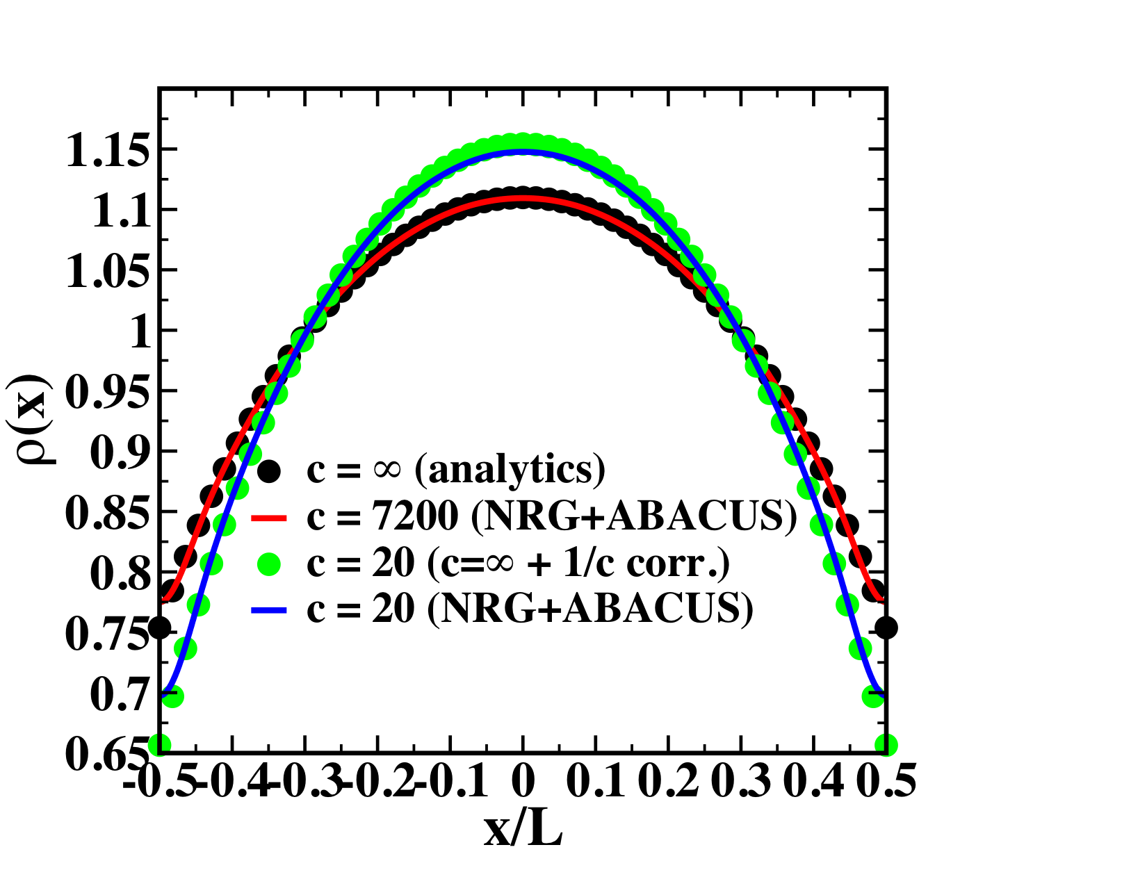
Harmonically trapped Lieb-Liniger
JSC & R. M. Konik, Phys. Rev. Lett. 109, 175301 (2012)
Interaction quench: GSE from NRG + TSA
Neil Robinson, Bart de Klerk + JSC, SciPost Phys. 11, 104 (2021)
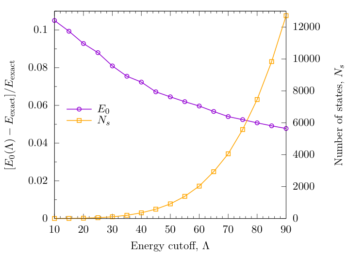
Ground-state energy from NRG + TSA
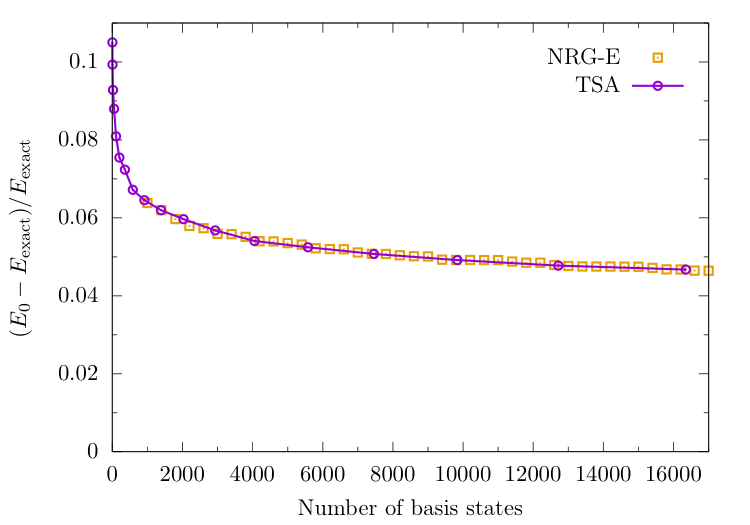
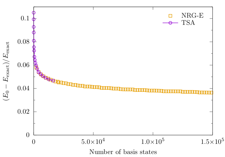
$N_s=600$ and $\Delta N_s = 200$ (corresponding to an initial energy cutoff of $\Lambda \approx 50$)
NRG follows TSA, but can include many more states.
Is ordering in energy a good idea?
Let's try an alternative metric...
We will order by matrix element size, between states in computational basis and the 3 lowest-lying ones from TSA:
$ \left| \langle \{\lambda\}^{(n)}_N | g_2(0) | \tilde E_j\rangle \right|, ~~j =0,1,2. $
NRG-E versus NRG-ME
Energy ordering versus Matrix Element ordering
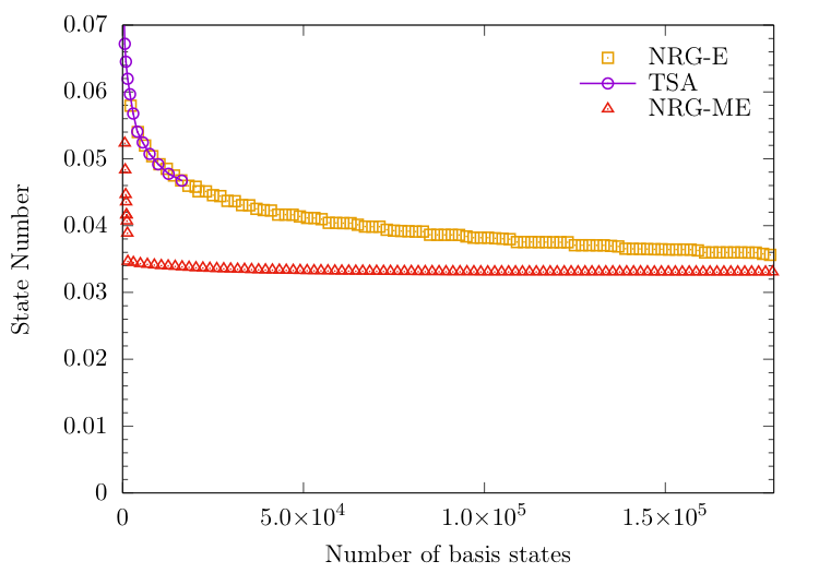
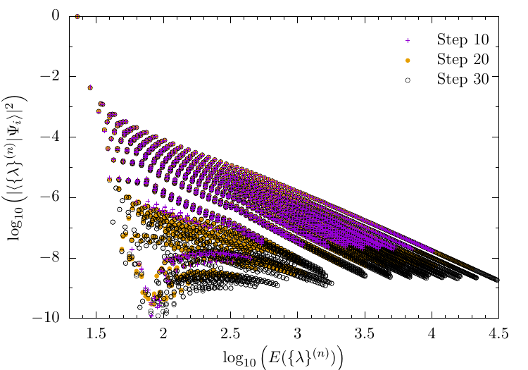
NRG-ME: convergence of the overlaps
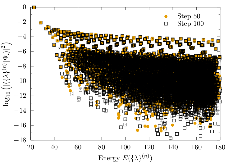
Highest overlap states
Earlier ME ordering
Towards a "perfect" ordering
ABACUS is really efficient at computing
dynamical correlation functions
For an operator ${\cal O}$, it preferentially seeks states with high matrix elements $ \langle \{\lambda\}^{(0)}_N | {\cal O} | \{\lambda\}^{(n)}_N\rangle $
Strategy: use ABACUS idea but with metric
$ w\left(|\{\lambda\}^{(n)}_N\rangle\right) = \left\vert \frac{\langle \{\lambda\}^{(n)}_N | g_2(0) | \{\lambda\}^{(0)}_N\rangle}{ E(\{\lambda\}^{(n)}_N) - E(\{\lambda\}^{(0)}_N) + \epsilon}\right\vert $
which favours the lower end of the spectrum
($\epsilon$ is set to $0.1$ to avoid $(n)=(0)$ divergence)
HOSTS: High Overlap States Truncation Scheme

This produces an ordering which is similar to the "back-engineered" one from the overlaps:
Energy convergence using HOSTS
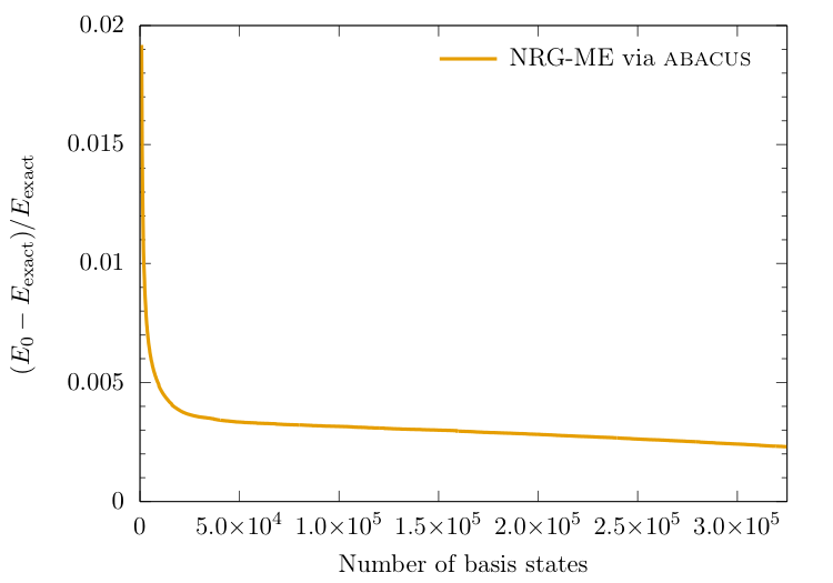
- ABACUS short run
- 390K states generated
- preferentially ordered
- NRG performed with $N_{NRG}=800$ and $\Delta N = 160$
- Convergence of $E_0$ to under 1% achieved with only a few thousand basis states
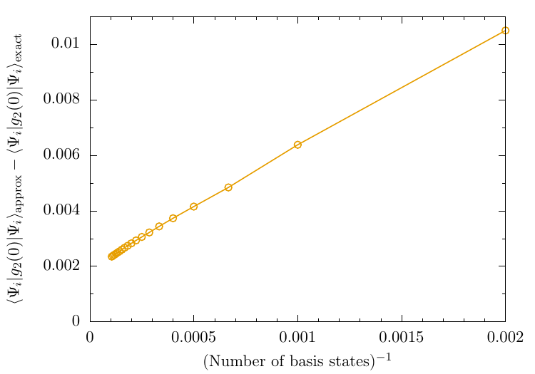
Convergence of other quantities using HOSTS
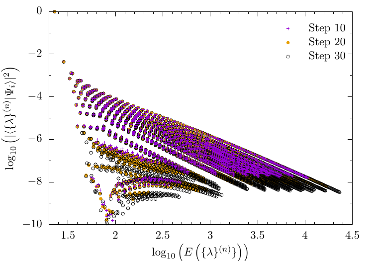
Overlaps
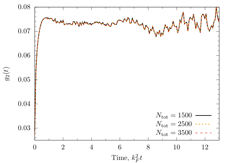
Local expectation value: $g_2$
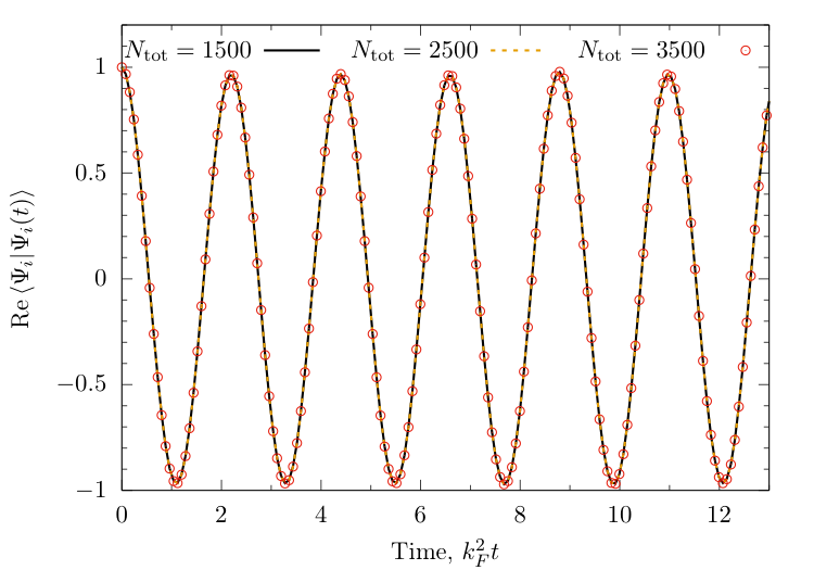
Real-time dynamics after the quench
Return amplitude
$ \langle \Psi_i |\Psi_i(t)\rangle \approx \sum_{n=0}^{N_{\text{tot}}} e^{-\mathrm{i}E(\{\lambda\}^{(n)}t} \left\vert \langle \{\lambda\}^{(n)} | \Psi_i \rangle \right\vert^2 $
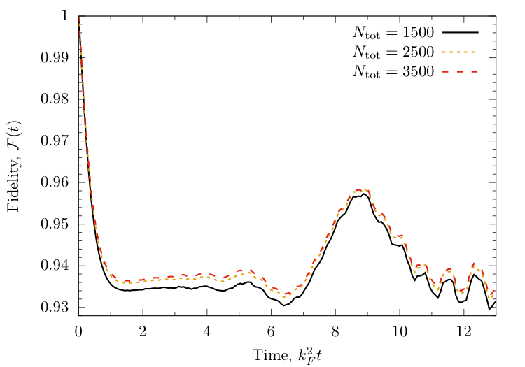
Fidelity
$ {\cal F}(t) = |\langle\Psi_i|\Psi_i(t)\rangle|^2 $
Time dependence of local observables
$ \begin{align} \langle &O(t)\rangle_i \equiv \langle \Psi_i(t) | O |\Psi_i(t)\rangle\\ & = \sum_{n,m=0}^{N_\text{tot}} e^{-\mathrm{i}t[E(\{\lambda\}^{(n)}) - E(\{\lambda\}^{(m)})]} \langle \Psi_i | \{ \lambda \}^{(m)} \rangle \langle \{ \lambda \}^{(m)} | O |\{\lambda\}^{(n)} \rangle \langle \{\lambda\}^{(n)} | \Psi_i\rangle \end{align} $
Although pretty successful, our alternative ordering still somehow relies on the perturbation being weak.
Desire: describe strongly non-perturbative quenches.
Challenge: account for contributions from important intermediate states.
Idea: keep approximate states at each step of the NRG, and select at each individual step which ones should participate, based on quadratic approximation of perturbative series.
$\rightarrow$ Matrix Element Renormalization
Matrix Element Renormalization
The overall workflow (steps 1-3 / 7):
- Generate the computational basis via preferential state generation from the seed state $|\Omega \rangle$. Order the states in the computational basis according to the metric "ME over Ediff" to obtain $\{|\{\lambda\}^{(j)}\rangle \}$.
- Construct a truncated Hamiltonian from the first $N_s+\Delta N_s$ computational basis states, $\big\{ |\{\lambda\}^{(1)}\rangle, \ldots, |\{\lambda\}^{(N_s+\Delta N_s)}\rangle\big\}$ and diagonalize this Hamiltonian to obtain the first approximate eigenstates $\big\{|1\rangle, \ldots , |N_s+\Delta N_s\rangle\big\}$ with energies $\{ E_1, \ldots, E_{N_s + \Delta N_s} \}$.
- Compute the overlaps between $|\{\lambda\}^{(0)}\rangle$ and the newly acquired approximate eigenvectors $\{|1\rangle, \ldots, |N_s + \Delta N_s\rangle \}$. Then relabel the approximate eigenstates such that $|1\rangle$ refers to the approximate eigenstate with the largest overlap.
Matrix Element Renormalization
The overall workflow (step 4 / 7):
- Take the next $\Delta N_s$ computational basis states $|\{\lambda\}^{(j)}\rangle$ and compute the second order weight for each of the approximate eigenstates $|i \rangle$ with $i>1$ obtained in previous steps: \[ w_2\left( |i \rangle \right) = \sum_{j} \frac{ \langle i | \delta H |\{\lambda\}^{(j)} \rangle \langle \{\lambda\}^{(j)} | \delta H | 1 \rangle}{( E_1 - E_{\{\lambda\}}^{(j)}) (E_1 - E_i)}. \] Here $\delta H = cR\times g_2(0)$ is the perturbing operator, the sum ranges over all the newly added computational basis states, and $E_{\{\lambda\}}^{(j)} = E(\{\lambda\}^{(j)})$ are the energies of the newly added computational basis states.
Matrix Element Renormalization
The overall workflow (steps 5 - 7 / 7):
- Form a truncated basis consisting of $|1\rangle$, the $N_s-1$ states in $\{|i \rangle \big\}_{i>1}$ with the largest $w_2$-weight, and the $\Delta N_s$ computational basis states introduced in step 4, construct the truncated Hamiltonian in this basis and diagonalize it to obtain $N_s + \Delta N_s$ new approximate eigenstates $\{|1'\rangle, \ldots, |(N_s + \Delta N_s)'\rangle\}$.
- Compute the overlaps between $|1\rangle$ and the newly acquired approximate eigenvectors, and replace $|1\rangle$ by the approximate eigenvector with the largest overlap. Replace the remaining approximate eigenvectors used to form the truncated basis in step 5 with the remaining newly obtained approximate eigenvectors.
- Return to the fourth step.
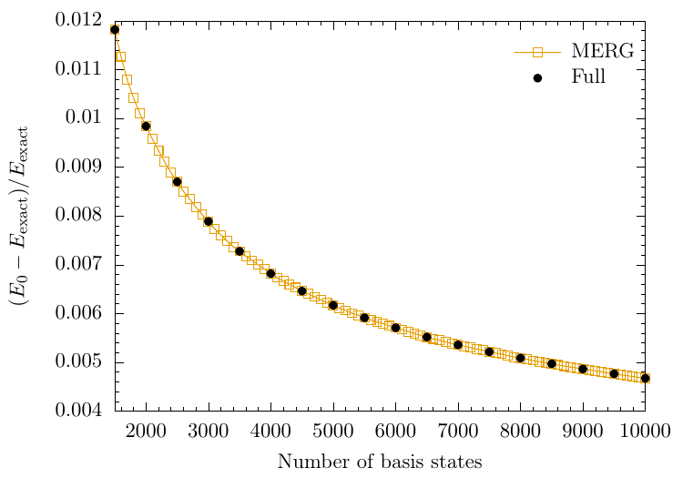
Convergence using MERG
Overlaps
Energy
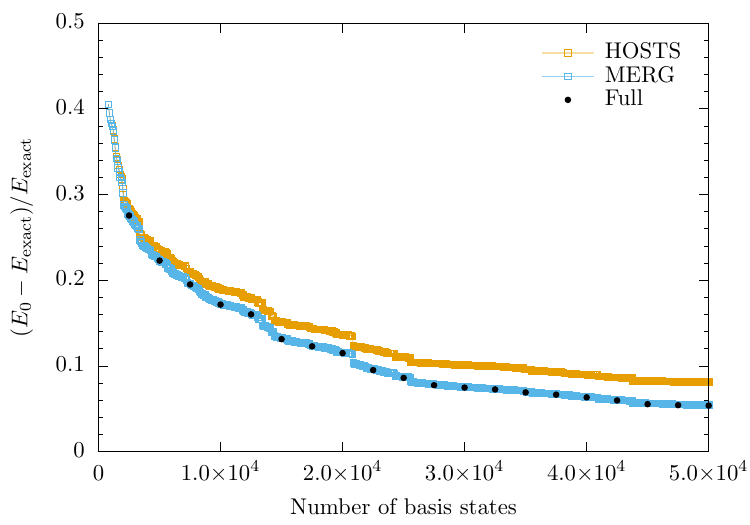
MERG for a harder quench
Conclusions and perspectives
- Integrable models as a basis for renormalization: without doubt a good idea
- Matrix elements for many cases are available
- Ordering by energy is demonstrably suboptimal
- Order(s?) of magnitude improvements in computational efficiency obtainable by using more refined measures $\rightarrow$ new take on RG
Generalized Hydrodynamics
Quenches from spatially inhomogeneous states
- B. Bertini, M. Collura, J. De Nardis and M. Fagotti, PRL 117, 207201 (2016)
- O. A. Castro-Alvaredo, B. Doyon and T. Yoshimura, PRX 6, 041065 (2016)
- B. Doyon and T. Yoshimura, SciPost Phys. 2, 014 (2017)
After initial dephasings: 'hydrodynamic' evolution described by local GGE
$\partial_t \rho (\lambda) + \partial_x (v^{\tiny \mbox{eff}}(\lambda) \rho (\lambda)) = 0$
with effective velocities determined by the dressing equation
Effective dynamics:
"flea gas" of scattering quasiparticles
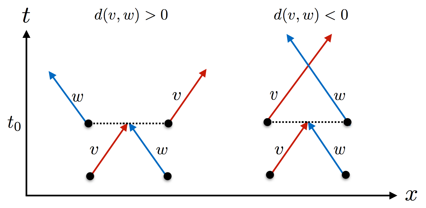
Flea gas GHD
for the Quantum Newton's Cradle
JSC, B. Doyon, J Dubail, R. Konik and T. Yoshimura, SciPost Phys. 6, 070 (2019)
Short time scales:
Flea gas GHD
for the Quantum Newton's Cradle
JSC, B. Doyon, J Dubail, R. Konik and T. Yoshimura, SciPost Phys. 6, 070 (2019)
Longer time scales:
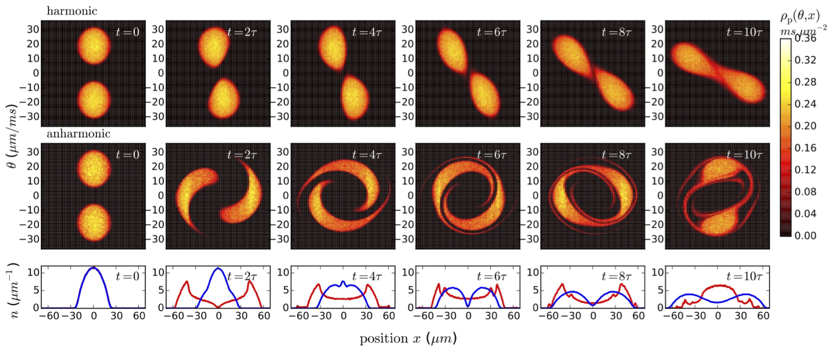
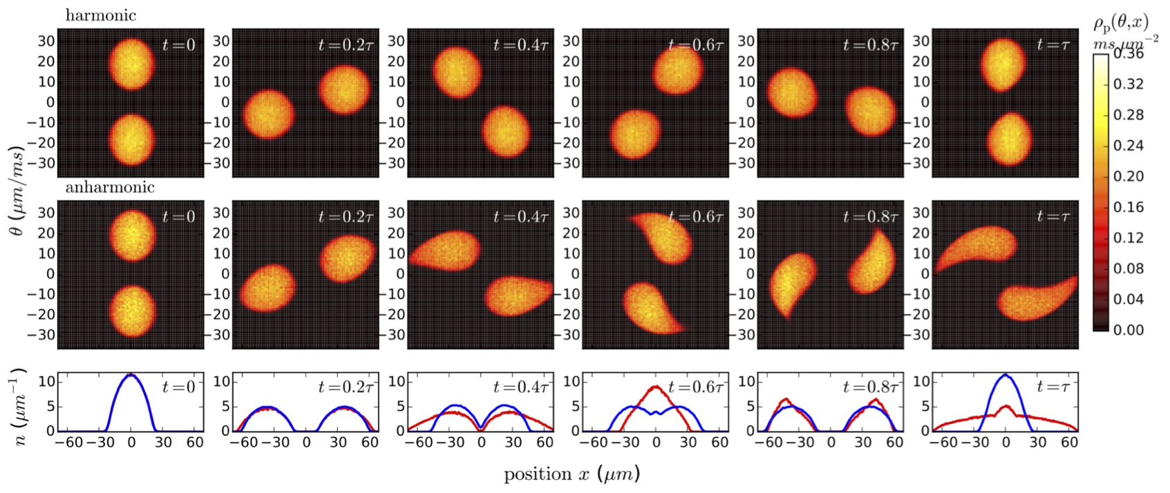
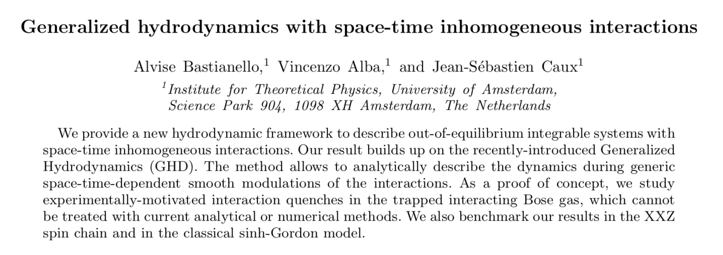
Generalized Hydrodynamics with space/time-dependent potentials
Phys. Rev. Lett. 123, 130602 (2019)
Adiabatic formation of bound states in the 1d Bose gas
Phys. Rev. B 103, 165121 (2021)
Spin Chain Bonus
The structure factor
of the Heisenberg chain
Quantum wake dynamics in Heisenberg
A. Scheie, P. Laurell, B. Lake, S. E. Nagler, M. B. Stone, JSC, D. A. Tennant
- Inelastic neutron scattering on $K Cu F_3$
- Really accurate data in momentum/frequency space enabling...
- Fourier transform to real space / time
- Look specifically at high-energy features
- Quantum wake: a local, coherent, long-lived, quasiperiodically oscillating magnetic state emerging out of the distillation of propagating excitations following a local quantum quench
Quantum wake dynamics in Heisenberg
Quantum wake dynamics in Heisenberg
Quantum wake dynamics in Heisenberg
Selectively (patch-wise) Fourier transforming shows that the $k=\pi/2$ (mod $2\pi$) states are responsible for the quantum wake dynamics
These effects are beyond the reach of any low-energy method