Integrability
and truncated spectrum approach
for out-of-equilibrium dynamics
10th Bologna Workshop
on Conformal Field Theory and Integrable Models
Bologna, 6 September 2023
Jean-Sébastien Caux


Plan of the talk
Out-of-equilibrium: why?
Why NOT?
- Real systems equilibrate very rapidly
- Experimentally: tough to control
- Theoretically: can't do it - toolbox too limited
Why INDEED?
- Real isolated systems can equilibrate slowly
- Novel states & properties
- Experimentally: frontier of current capabilities
- Theoretically: the toughest challenge around?
Mechanical
motivation
Out of equilibrium: categories
- local, gentle (linear response)
- local, hard (nonlinear response)
- local, gentle, repeated
- local, hard, repeated
- local, gentle, erratic
- local, hard, erratic
- extended, one-time
- extended, repeated regularly
- extended, erratic
Out of equilibrium: terminology
Out of equilibrium: what? how?
- Neutron scattering
- Bragg spectroscopy
- Transport
- Linear response
- Traditional methods
- CFT, Bosonization, ...
- Magnetic resonance
- Photoemission
- Ultrafast spectr.
- Free models
- Numerics
- Nonlinear response theory
- Feshbach resonances
- Integrability
- Hydrodynamics ($t\rightarrow \infty$)
- GGE ($t = \infty$)
- Quench Action ($\forall t$)
- Masers/lasers
- Resonators
- Free models
- Floquet theory
- Numerics
- Despair?
Out-of-equilibrium using Integrability
- Split Fermi seas (Moses states)
- Spin echo in quantum dots
- Quasisolitons
- The super Tonks-Girardeau gas
- Interaction quench in Richardson
- Domain wall release in Heisenberg
- Geometric quench
- Interaction cutoff in Lieb-Liniger
- Release of trapped Lieb-Liniger
- BEC to Lieb-Liniger quench
- Quantum Newton’s Cradle in TG
- Néel to XXZ quench
- Generalized hydrodynamics
- Floquet driven spin chains
The Lieb-Liniger Model
$ H = \int_0^L dx \left[ \partial_x \Psi^{\dagger}(x) \partial_x \Psi(x) + c \Psi^{\dagger} (x) \Psi^{\dagger}(x) \Psi(x) \Psi(x) \right] $
Eigenstates: Bethe Ansatz
\[ \begin{align} \Psi_N(\{ x \} | \{ \lambda \}) &= \prod_{N \geq j_1 > j_2 \geq 1} sgn(x_{j_1} - x_{j_2}) sgn (\lambda_{j_1} - \lambda_{j_2}) \times \\ &\times \sum_{P \in \pi_N} (-1)^{[P]} e^{i \sum_{j=1}^N \lambda_{P_j} x_j + \frac{i}{2} \sum_{N \geq j_1 > j_2 \geq 1} sgn(x_{j_1} - x_{j_2}) \phi (\lambda_{P_{j_1}} - \lambda_{P_{j_2}})} \end{align} \]
in which $\phi(\lambda) \equiv 2\mbox{atan}(\lambda/c)$
The Lieb-Liniger Model
Rapidities must obey the Bethe equations:
$ e^{\mathrm{i}\lambda_j L} = \prod_{\substack{{\tiny l=1} \\ {\tiny (l\neq j)}}}^{\tiny N} \frac{ \lambda_j - \lambda_l + \mathrm{i}c}{\lambda_j - \lambda_l - \mathrm{i}c} $
Eigenvalues of conserved charges:
$ Q_n\left(\{\lambda\}_N\right) = \sum_{j=1}^N \lambda_j^n, \quad n = 1,2,\ldots $
with in particular $P = Q_1, E = Q_2$.
The Lieb-Liniger Model
Description using the Algebraic Bethe Ansatz
\[ \tau(\lambda) = tr T(\lambda), \hspace{5mm} T(\lambda) = \left( \begin{array}{cc} A(\lambda) & B(\lambda) \\ C(\lambda) & D(\lambda) \end{array} \right), \hspace{5mm} | \Psi_N \left( \left\{ \lambda \right\}_N \right \rangle = \prod_j B(\lambda_j) | 0 \rangle \]
Matrix elements of physical operators known from:
- Gaudin formula for state norm
\[ \langle \{ \lambda \} | \{ \lambda \} \rangle = c^N \prod_{j > k} \frac{\lambda_{jk}^2 + c^2}{\lambda_{jk}^2} \mbox{det} \left[ \delta_{jk} \left(L + \sum_l K_{jl} \right) - K_{jk} \right], \hspace{10mm} K_{jk} = \frac{2c}{\lambda_{jk}^2 + c^2} \]
- solution of inverse problem $A, B, C, D \leftrightarrow \psi(x), \psi^\dagger(x)$
- Slavnov formula for $\langle 0 | \prod_j C(\lambda_j) \prod_k B(\mu_k) | 0 \rangle$
The Lieb-Liniger Model
(Dynamical) Correlation functions
\[ {\cal S}^{a \bar{a}} (k, \omega) \equiv \frac{1}{N} \sum_{j, j'} e^{-i k(j-j')} \int_{-\infty}^\infty dt e^{i\omega t} \langle \frac{1}{2} \left[ {\cal O}^a_j (t), ({\cal O}^a_{j'} (0))^\dagger \right] \rangle \]
Simplest examples:
- Dynamical structure factor: ${\cal O}_j = \rho_j \equiv \Psi^\dagger(x_j) \Psi(x_j)$
- One-body function (Green's): ${\cal O}_j = \Psi(x_j)$ or $\Psi^\dagger(x_j)$
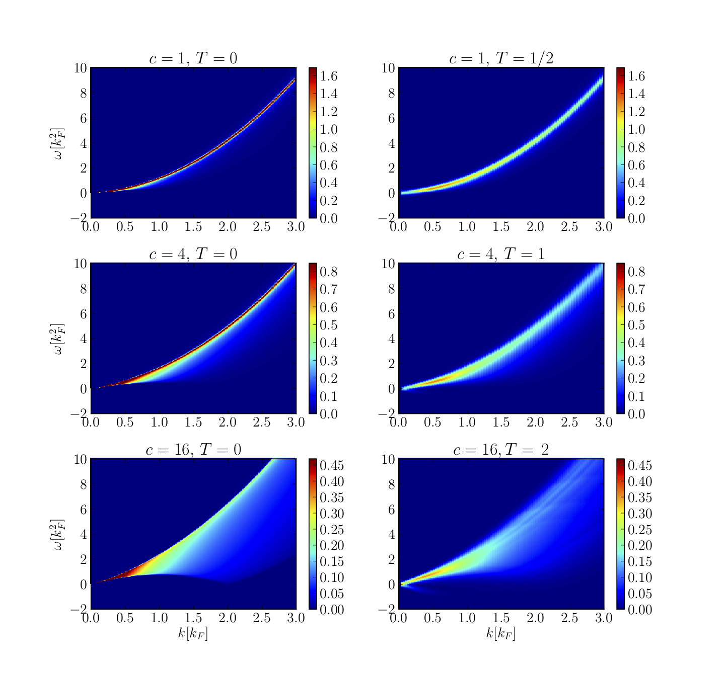
Dynamical structure factor
from (algebraic) Bethe Ansatz

Dynamical structure factor
from (algebraic) Bethe Ansatz
The ABACUS algorithm
Dynamical structure factor from Bethe Ansatz
extension to finite TM. Panfil and J-SC, PRA 89 (2014)
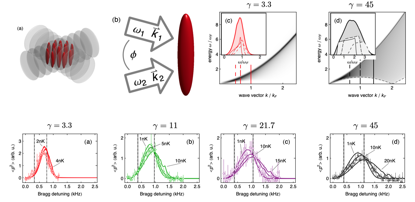
Lieb-Liniger using cold atoms (I)
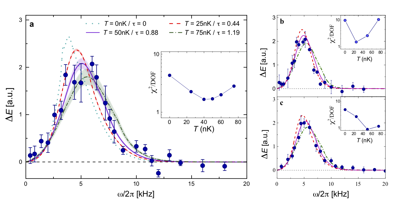
Lieb-Liniger using cold atoms (II)
Let's

Interaction quench in Lieb-Liniger
We will consider a sudden switch of the interaction:
$ c (t) = \left\{ \begin{array}{ll} c_i & t < 0, \\ c_f & t > 0 \end{array} \right. $
starting in ground/(any eigen)state of $H(c_i)$ at $t < 0$
For many reasons, this is a complicated problem...
- GGE logic fails, charges have $\infty$ exp. values
- approaches using regularizations (q-bosons, extended charges, ...): no complete solution
The strategy
We write the initial state in the basis of the eigenstates of $H(c_f)$, denoted as $\left\{ |\{\lambda\}^{(n)}_N\rangle \right\}, n = 0, 1, ...$
The initial state is obtained as a linear decomposition weighed by exact overlaps:
$ |\Psi_i\rangle = \sum_{n=0}^\infty |\{\lambda\}^{(n)}_N\rangle \underbrace{\langle \{\lambda\}^{(n)}_N | \Psi_i\rangle}_{\text{the overlaps}} $
Exact time-evolved state:
$ |\Psi_i(t)\rangle \equiv e^{-iH(c_f)t} |\Psi_i\rangle = \sum_{n=0}^\infty e^{-\mathrm{i}E(\{\lambda\}^{(n)}_N)t} |\{\lambda\}^{(n)}_N\rangle \langle \{\lambda\}^{(n)}_N | \Psi_i\rangle $
The Quench Action
Setup
The initial state is decomposed in the basis of post-quench Hamiltonian eigenstates:
$ |\Psi (t=0) \rangle = \sum_{\{ I \}} e^{-S^\Psi_{\{ I \}}} | \{ I \} \rangle, $
with overlaps encoded in the coefficients$ S^\Psi_{\{ I \}} = -\ln \langle \{ I \} | \Psi (t=0) \rangle ~\in ~\mathbb{C} $
Exact time-dependend expectation values:
$ \bar{\cal O} (t) = \frac{ \sum_{\{ I^l \} } \sum_{\{ I^r\}} e^{-(S^\Psi_{\{ I^l\}})^* - S^\Psi_{\{ I^r\}} + i (\omega_{\{ I^l\}} - \omega_{\{ I^r\}})t} \langle \{ I^l \}| {\cal O} | \{ I^r \} \rangle}{\sum_{\{ I \}} e^{-2\Re S^\Psi_{\{ I \}}}} $
Going to the thermodynamic limit
Summations over eigenstates are replaced by functional integrals
$ \lim_{Th,reg} \sum_{\{ \rho_i \}} (...) = \int_{\rho_{sm} \in C^\infty} D\rho_{sm} (...) $
Normalization sum (trivially 1) represented as
$ \lim_{Th,reg} \langle \Psi (t) | \Psi (t) \rangle = \int D\rho_{sm} ~ e^{-S^Q[\rho_{sm}]} $
where the Quench Action is defined as
$ S^{Q}[\rho] = S^o[\rho] - S^{YY}[\rho] $
Time-dependent expectation values
In ThLim, saddle-point evaluation $\left. \frac{\delta S^Q[\rho]}{\delta \rho} \right|_{\rho_{sp}} = 0$ exactly gives the full time evolution of observables as
$ \begin{align} \lim_{Th,reg} \bar{\cal O} (t) = \lim_{Th,reg} \frac{1}{2} \sum_{\bf e} \left[ e^{-\delta S_{\bf e}[\rho_{sp}] - i \omega_{\bf e}[\rho_{sp}] t} \langle \rho_{sp} | {\cal O} | \rho_{sp}; {\bf e} \rangle \right. \nonumber \\ \left. + e^{-\delta S^*_{\bf e}[\rho_{sp}] + i \omega_{\bf e}[\rho_{sp}] t} \langle \rho_{sp}; {\bf e} | {\cal O} | \rho_{sp} \rangle \right] \end{align} $
provided the
operator ${\cal O}$ is
- weak
- smooth
- thermodynamically finite
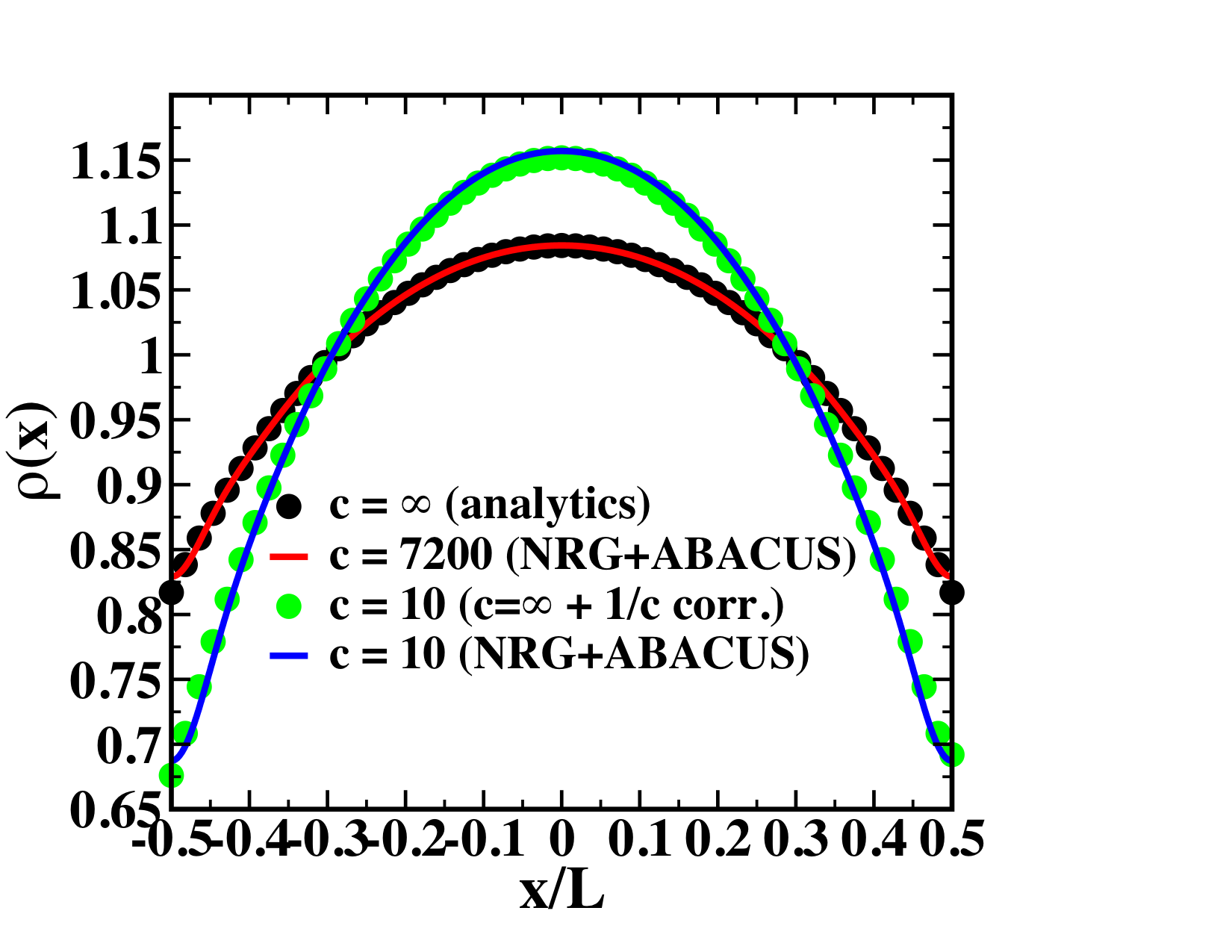
The BEC to Lieb-Liniger quench
Initial state: ground state of free bosons
$ | \Psi_0 \rangle = \frac{1}{\sqrt{L^N N!}} \left(\psi_{k=0}^\dagger\right)^N | 0 \rangle $
Exact overlaps with finite $c$ Lieb-Liniger states:
$ \langle \Psi_0 | \{ \lambda \}_{N/2} \cup \{ -\lambda \}_{N/2} \rangle = \left[ \frac{(cL)^{-N} N!}{\mbox{det}_N G_{jk} }\right]^{1/2} \frac{\mbox{det}_{N/2} G^Q_{jk}}{\prod_{j=1}^{N/2} \frac{\lambda_j}{c} \left[ \frac{\lambda_j^2}{c^2} + \frac{1}{4} \right]^{1/2}} $
in which $G_{jk}$ is the Gaudin matrix
$ G_{jk} = \delta_{jk} \left[ L + \sum_{l=1}^N K (\lambda_j, \lambda_l) \right] - K(\lambda_j, \lambda_k) $
Exact solution using Quench Action
$ S^Q = L\int_0^\infty d\lambda \rho(\lambda) \log\left(\frac{\lambda^2}{c^2} \left( \frac{1}{4} + \frac{ \lambda^2}{c^2} \right) \right) + S^{YY} $
Saddle-point equation:
$ \ln \eta(\lambda) = g(\lambda) - h - \int_{-\infty}^\infty \frac{d\lambda'}{2\pi} K (\lambda - \lambda') \ln \left[ 1 + \eta^{-1}(\lambda') \right], $
with driving term $ g(\lambda) = \ln \left[ \frac{\lambda^2}{c^2} \left( \frac{\lambda^2}{c^2} + \frac{1}{4} \right) \right] $
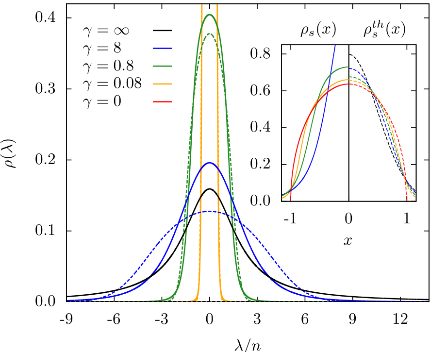
Analytic solution for steady state:
$ \begin{align} \rho_{sp} (\lambda) &= -\frac{\gamma}{4\pi} \frac{1}{1 + a(\lambda)} \frac{\partial a(\lambda)}{\partial \gamma},\\ a(\lambda) &\equiv \frac{2\pi}{\frac{\lambda}{n} \sinh \frac{2\pi \lambda}{c}} I_{1 - 2i\frac{\lambda}{c}} \left(\frac{4}{\sqrt{\gamma}}\right) I_{1 + 2i\frac{\lambda}{c}} \left(\frac{4}{\sqrt{\gamma}}\right) \end{align} $
Exact solution using Quench Action
Steady state distribution: non-thermal
J. De Nardis, B. Wouters, M. Brockmann & J-SC, PRA 89, 2014
Numerical Renormalization approach
to the interaction quench
in Lieb-Liniger
Neil Robinson, Bart de Klerk + JSC
Viewed as a perturbation
$ H(c_i) = H(c_f) + (c_i - c_f) \int_0^L dx \Psi^\dagger(x)\Psi^\dagger(x)\Psi(x)\Psi(x) $
Matrix elements of the original Hamiltonian in the computational basis of post-quench eigenstates:
$ \begin{align} \langle \{\lambda\}^{(m)}_N | H(c_i) | \{\lambda\}^{(n)}_N \rangle &= \delta_{n,m} E\big(\{\lambda\}^{(n)}_N \big) + \\ &+ (c_i - c_f) L\, \langle \{\lambda\}^{(m)}_N | \big(\Psi^\dagger(0)\big)^2 \big( \Psi(0) \big)^2 |\{\lambda\}^{(n)}_N\rangle \end{align} $
Said otherwise, we perturb the system
with the operator
$ g_2(0) = \big( \Psi^\dagger(0)\big)^2 \big(\Psi(0)\big)^2 $
Truncated Spectrum Approach
Idea: truncate Hilbert space to low-E sector using cutoff $\Lambda$, then diagonalize numerically
NRG + TSA
The overall workflow:
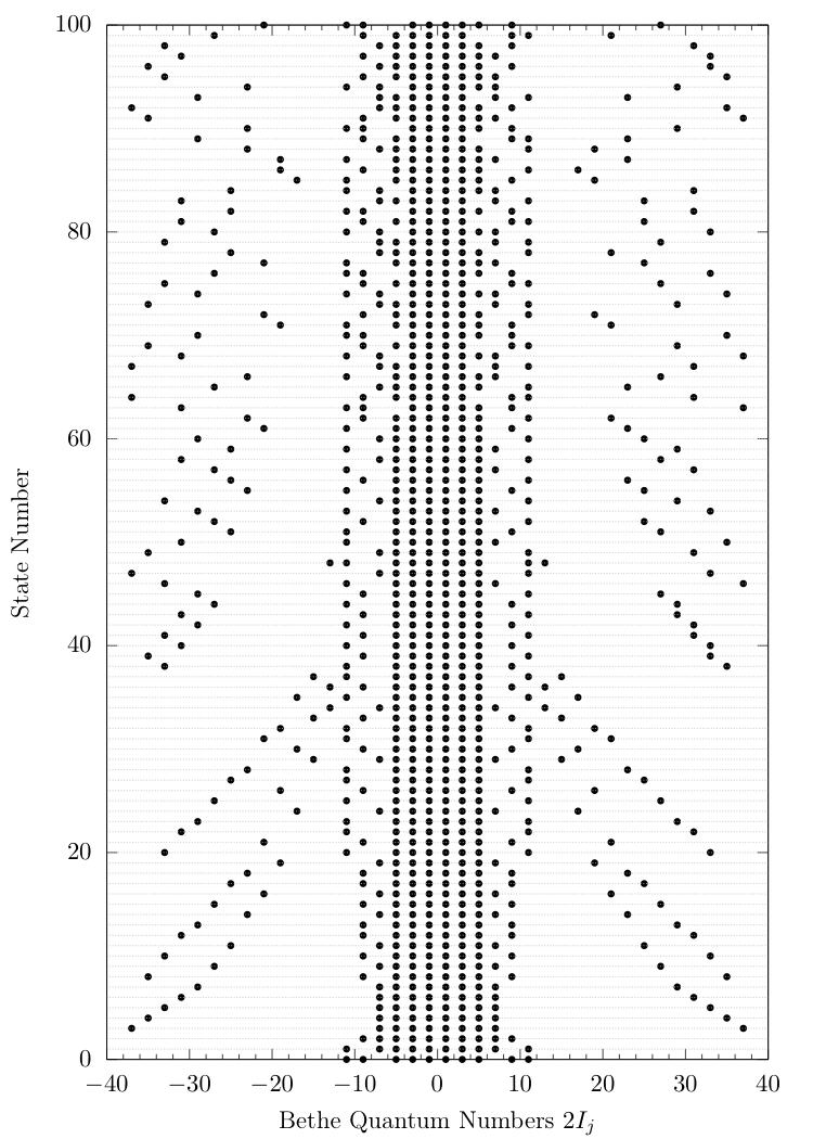
- Construct the computational basis $\{ |\{\lambda\}^{(j)}\rangle\}$ and order by energy $E(\{\lambda\}^{(j)})$
- Construct the Hamiltonian with the lowest $N_s+\Delta N_s$ states: $ \begin{align} \Big\{ |\{\lambda\}^{(1)}\rangle, \ldots, |\{\lambda\}^{(N_s+\Delta N_s)}\rangle\Big\}, \end{align} $ and diagonalize it, obtaining approximate energies and eigenstates $ \begin{align} \Big\{ |E^{(1)}\rangle, \ldots , |E^{(N_s+\Delta N_s)}\rangle \Big\}. \end{align} $
- Discard the highest $\Delta N_s$ approximate eigenstates $ \begin{align} \Big\{|E^{(N_s+1)}\rangle,\ldots,|E^{(N_s+\Delta N_s)}\rangle\Big\}, \end{align} $ and form a new basis with the lowest $N_s$ approximate eigenstates and the next $\Delta N_s$ lowest states in the computational basis.
- Construct the Hamiltonian in the new basis, and diagonalize to obtain new approximate eigenstates.
- Return to the third step.
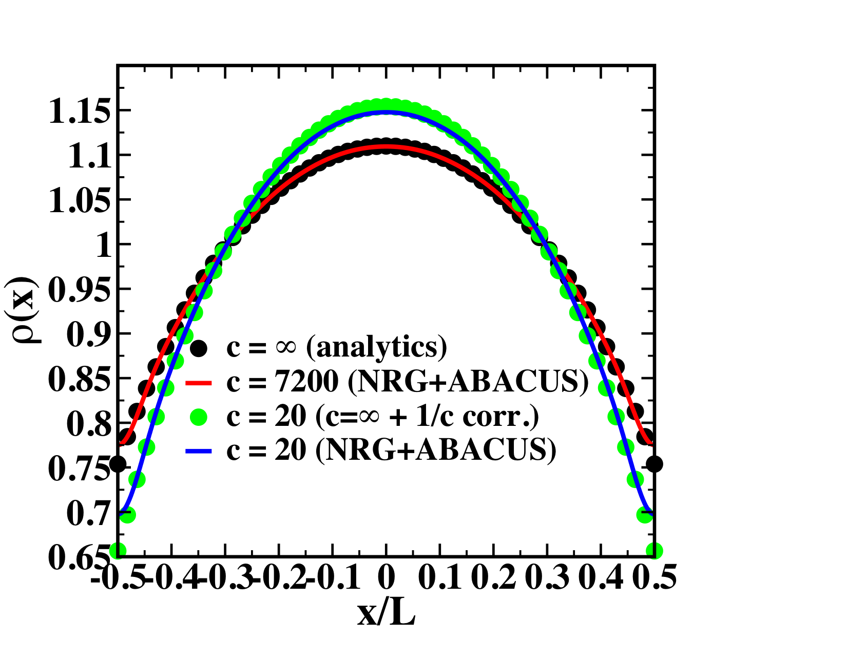
Harmonically trapped Lieb-Liniger
JSC & R. M. Konik, Phys. Rev. Lett. 109, 175301 (2012)
Interaction quench: GSE from NRG + TSA
Neil Robinson, Bart de Klerk + JSC, SciPost Phys. 11, 104 (2021)
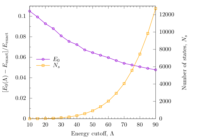
Ground-state energy from NRG + TSA
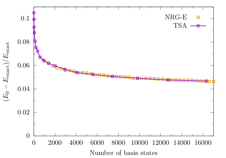
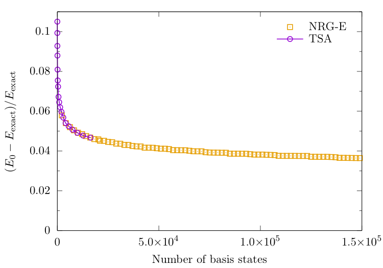
$N_s=600$ and $\Delta N_s = 200$ (corresponding to an initial energy cutoff of $\Lambda \approx 50$)
NRG follows TSA, but can include many more states.
Is ordering in energy a good idea?
Let's try an alternative metric...
We will order by matrix element size, between states in computational basis and the 3 lowest-lying ones from TSA:
$ \left| \langle \{\lambda\}^{(n)}_N | g_2(0) | \tilde E_j\rangle \right|, ~~j =0,1,2. $
NRG-E versus NRG-ME
Energy ordering versus Matrix Element ordering
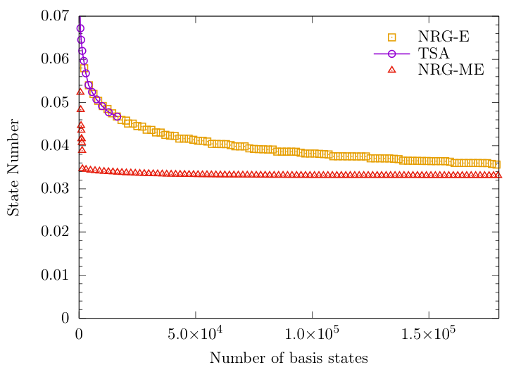
NRG-ME: convergence of the overlaps
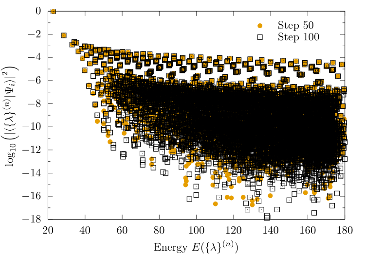
Highest overlap states
Earlier ME ordering
Towards a "perfect" ordering
ABACUS is really efficient at computing
dynamical correlation functions
For an operator ${\cal O}$, it preferentially seeks states with high matrix elements $ \langle \{\lambda\}^{(0)}_N | {\cal O} | \{\lambda\}^{(n)}_N\rangle $
Strategy: use ABACUS idea but with metric
$ w\left(|\{\lambda\}^{(n)}_N\rangle\right) = \left\vert \frac{\langle \{\lambda\}^{(n)}_N | g_2(0) | \{\lambda\}^{(0)}_N\rangle}{ E(\{\lambda\}^{(n)}_N) - E(\{\lambda\}^{(0)}_N) + \epsilon}\right\vert $
which favours the lower end of the spectrum
($\epsilon$ is set to $0.1$ to avoid $(n)=(0)$ divergence)
HOSTS: High Overlap States Truncation Scheme

This produces an ordering which is similar to the "back-engineered" one from the overlaps:
Energy convergence using HOSTS
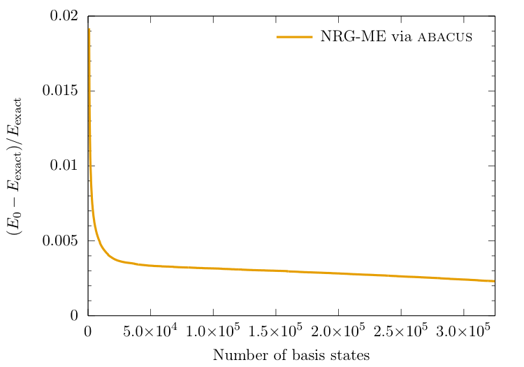
- ABACUS short run
- 390K states generated
- preferentially ordered
- NRG performed with $N_{NRG}=800$ and $\Delta N = 160$
- Convergence of $E_0$ to under 1% achieved with only a few thousand basis states
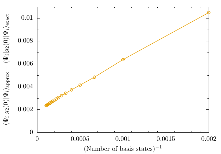
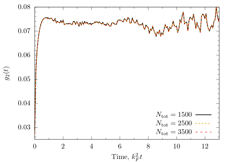
Convergence of other quantities using HOSTS
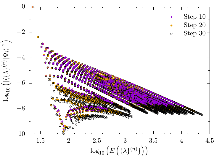
Overlaps
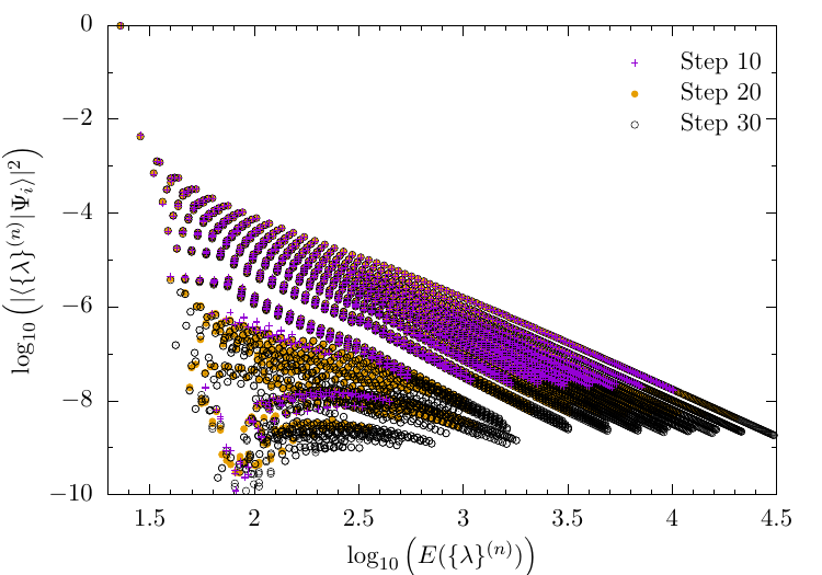
Local expectation value: $g_2$
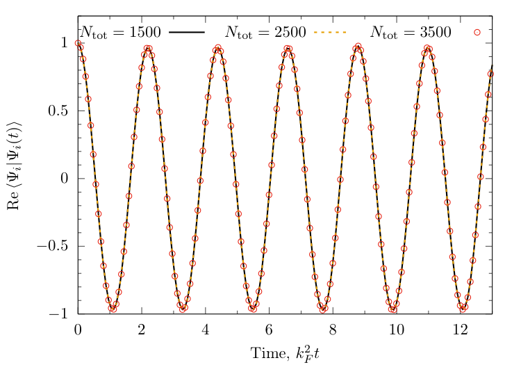
Real-time dynamics after the quench
Return amplitude
$ \langle \Psi_i |\Psi_i(t)\rangle \approx \sum_{n=0}^{N_{\text{tot}}} e^{-\mathrm{i}E(\{\lambda\}^{(n)}t} \left\vert \langle \{\lambda\}^{(n)} | \Psi_i \rangle \right\vert^2 $
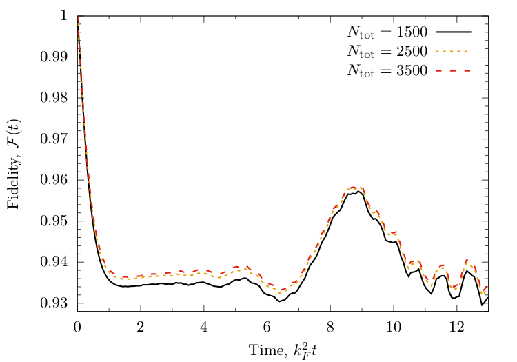
Fidelity
$ {\cal F}(t) = |\langle\Psi_i|\Psi_i(t)\rangle|^2 $
Time dependence of local observables
$ \begin{align} \langle &O(t)\rangle_i \equiv \langle \Psi_i(t) | O |\Psi_i(t)\rangle\\ & = \sum_{n,m=0}^{N_\text{tot}} e^{-\mathrm{i}t[E(\{\lambda\}^{(n)}) - E(\{\lambda\}^{(m)})]} \langle \Psi_i | \{ \lambda \}^{(m)} \rangle \langle \{ \lambda \}^{(m)} | O |\{\lambda\}^{(n)} \rangle \langle \{\lambda\}^{(n)} | \Psi_i\rangle \end{align} $
Although pretty successful, our alternative ordering still somehow relies on the perturbation being weak.
Desire: describe strongly non-perturbative quenches.
Challenge: account for contributions from important intermediate states.
Idea: keep approximate states at each step of the NRG, and select at each individual step which ones should participate, based on quadratic approximation of perturbative series.
$\rightarrow$ Matrix Element Renormalization
Matrix Element Renormalization
The overall workflow (steps 1-3 / 7):
- Generate the computational basis via preferential state generation from the seed state $|\Omega \rangle$. Order the states in the computational basis according to the metric "ME over Ediff" to obtain $\{|\{\lambda\}^{(j)}\rangle \}$.
- Construct a truncated Hamiltonian from the first $N_s+\Delta N_s$ computational basis states, $\big\{ |\{\lambda\}^{(1)}\rangle, \ldots, |\{\lambda\}^{(N_s+\Delta N_s)}\rangle\big\}$ and diagonalize this Hamiltonian to obtain the first approximate eigenstates $\big\{|1\rangle, \ldots , |N_s+\Delta N_s\rangle\big\}$ with energies $\{ E_1, \ldots, E_{N_s + \Delta N_s} \}$.
- Compute the overlaps between $|\{\lambda\}^{(0)}\rangle$ and the newly acquired approximate eigenvectors $\{|1\rangle, \ldots, |N_s + \Delta N_s\rangle \}$. Then relabel the approximate eigenstates such that $|1\rangle$ refers to the approximate eigenstate with the largest overlap.
Matrix Element Renormalization
The overall workflow (step 4 / 7):
- Take the next $\Delta N_s$ computational basis states $|\{\lambda\}^{(j)}\rangle$ and compute the second order weight for each of the approximate eigenstates $|i \rangle$ with $i>1$ obtained in previous steps: \[ w_2\left( |i \rangle \right) = \sum_{j} \frac{ \langle i | \delta H |\{\lambda\}^{(j)} \rangle \langle \{\lambda\}^{(j)} | \delta H | 1 \rangle}{( E_1 - E_{\{\lambda\}}^{(j)}) (E_1 - E_i)}. \] Here $\delta H = cR\times g_2(0)$ is the perturbing operator, the sum ranges over all the newly added computational basis states, and $E_{\{\lambda\}}^{(j)} = E(\{\lambda\}^{(j)})$ are the energies of the newly added computational basis states.
Matrix Element Renormalization
The overall workflow (steps 5 - 7 / 7):
- Form a truncated basis consisting of $|1\rangle$, the $N_s-1$ states in $\{|i \rangle \big\}_{i>1}$ with the largest $w_2$-weight, and the $\Delta N_s$ computational basis states introduced in step 4, construct the truncated Hamiltonian in this basis and diagonalize it to obtain $N_s + \Delta N_s$ new approximate eigenstates $\{|1'\rangle, \ldots, |(N_s + \Delta N_s)'\rangle\}$.
- Compute the overlaps between $|1\rangle$ and the newly acquired approximate eigenvectors, and replace $|1\rangle$ by the approximate eigenvector with the largest overlap. Replace the remaining approximate eigenvectors used to form the truncated basis in step 5 with the remaining newly obtained approximate eigenvectors.
- Return to the fourth step.
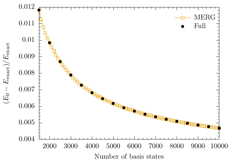
Convergence using MERG
Overlaps
Energy
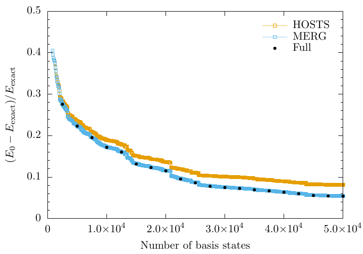
MERG for a harder quench
Conclusions and perspectives
- Integrable models as a basis for renormalization: without doubt a good idea
- Matrix elements for many cases are available
- Ordering by energy is demonstrably suboptimal
- Order(s?) of magnitude improvements in computational efficiency obtainable by using more refined measures $\rightarrow$ new take on RG